In Module 1, we assembled our mathematical toolkit. Now it's time to ask a deeper question:
How can we encode an entire computation — every step, every intermediate value — into a single polynomial divisibility check?
We will follow a natural progression:
- Arithmetic Circuits — represent any computation as a graph of wires and gates.
- R1CS — translate that graph into algebraic constraints.
- Schwartz–Zippel Lemma — learn why checking one random point is enough.
- QAP — lift R1CS into polynomials, so satisfying constraints becomes divisibility.
- Knowledge of Exponent & Encrypted Arithmetic — hide all values so the verifier checks everything without seeing anything.
Running example. Throughout this module we use the computation . Simple enough to follow by hand, rich enough to illustrate every idea.
All Rust snippets in this module come from the companion repository github.com/bsaepfl/zksnarks-101-labs. Clone it locally if you want to run, tweak, or extend the code yourself — every cell on this page is pre-executed with the output shown directly below it.
1. Arithmetic Circuits
When we write , we think of it as a single formula. But a proof system executes it one operation at a time:
| Step | Operation | Result |
|---|---|---|
| Gate 1 | ||
| Gate 2 | ||
| Gate 3 | ||
| Gate 4 |
Every value is a wire (). The operations are gates. Both the prover (Philip) and the verifier (Veronica) know the circuit structure. But only Philip knows the wire values. Veronica only knows input and output .
The challenge: how can Philip prove he computed all intermediate values correctly, without Veronica re-doing the computation?
The Rust snippet below makes that circuit explicit. It hardcodes the gates for , evaluates them one by one, and records every intermediate wire value in the witness.
Key Observations
- Any computation can be broken into multiplication and addition gates.
- The number of multiplication gates determines the cost of the proof. Our circuit has 3 multiplication gates and 1 addition gate.
- The full list of wire values is called the witness.
2. Rank-1 Constraint Systems (R1CS)
To do algebra with a circuit, we turn it into equations. Every multiplication gate gives:
For our circuit:
The addition gate has not disappeared. It is a purely linear relation, so we can write it as:
In the compact matrix view below, we keep the three multiplicative rows explicit and then check this final linear relation separately. That is also the reason additions will look cheaper later on: they do not contribute a new multiplication constraint.
Matrix Representation
Collect all wire values into a witness vector:
The leading is there so constraints can include constant terms. Without it, rows could only describe linear combinations of witness wires. With it, a row can also encode expressions like or, more generally, things such as by putting the constant in the first column. Even in our example, the linear relation uses this idea.
With columns ordered as , the three multiplicative gates give the concrete matrices:
Each row corresponds to one multiplication gate, and each column corresponds to one witness entry. The addition gate still sits outside these three rows as the separate linear check .
Each multiplicative constraint becomes a row in . The R1CS is satisfied when, element-wise:
The R1CS is a clean algebraic representation. But checking it directly means one check per gate — millions of gates means millions of checks. We need something more succinct.
3. The Schwartz–Zippel Lemma
Two different polynomials of degree can agree on at most points. If we pick a random point from a field with elements:
For and , this probability is astronomically small.
Schwartz–Zippel Lemma. You can check polynomial equality everywhere by checking at just one random point.
4. Quadratic Arithmetic Programs (QAP)
A Quadratic Arithmetic Program is the polynomial form of our R1CS. Instead of checking each gate one by one, we encode the whole system into a few polynomials and reduce correctness to a single divisibility check.
This is the key compression step: many local circuit constraints become one global algebraic statement that we can later test at a secret random point.
The plan is:
- Assign gate the value
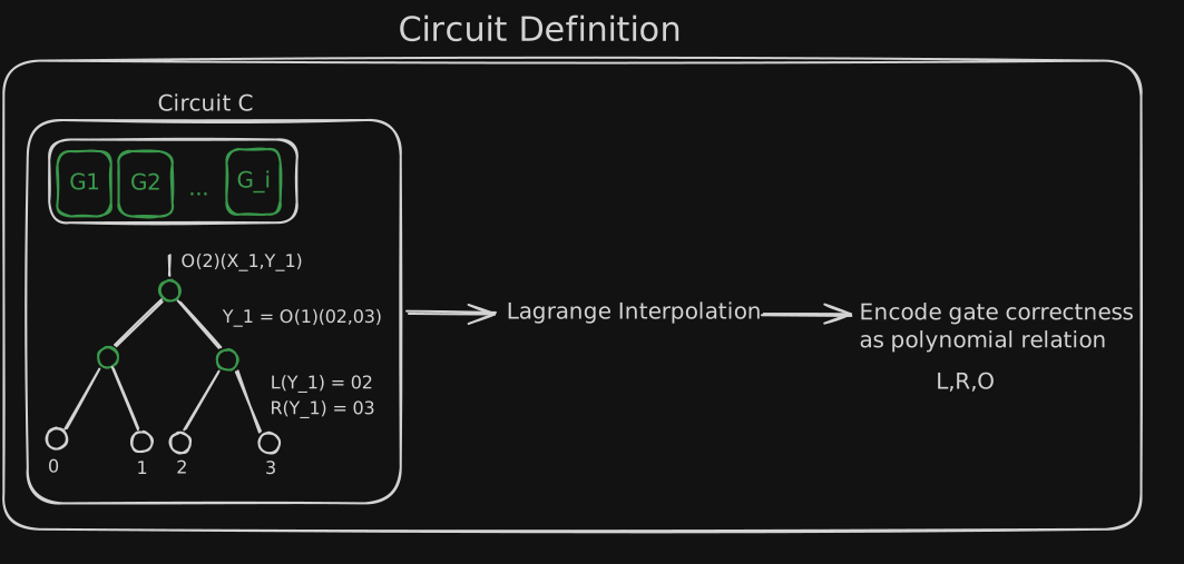
- Encode each column of the R1CS matrices as a polynomial via Lagrange interpolation
- Combine with wire values into
- Show that is divisible by if and only if all R1CS constraints are satisfied.
Step 1 — Gate Roots
Here the in is a formal polynomial variable, not the circuit input from . We use the points to label the three multiplication gates, so evaluating a polynomial at one of these values means “look at that gate”.
Step 2 — Sub-Polynomials
For each wire , define sub-polynomials by their values at each gate index:
The index tells us which witness wire we are talking about. The argument tells us which gate position we are querying. Concretely:
is the coefficient of wire on the left input of gate , is its coefficient on the right input, and is its coefficient on the output.
For example, has values because wire appears on the left side of gates 1 and 3, but not gate 2. Likewise, has values because wire is the output of gate 2 only.
This is exactly the link with the R1CS matrices: each sub-polynomial is obtained from one column of . For instance, the column of is , so interpolating those three gate values gives . The column of is , so it becomes .
So the QAP is not inventing new information: it is just turning each relevant matrix column into a polynomial that can be evaluated at gate positions. Columns that are all zero correspond to the zero polynomial and are usually omitted from the notation.
| Gate 1 | Gate 2 | Gate 3 | |
|---|---|---|---|
| 1 | 0 | 1 | |
| 0 | 1 | 0 | |
| 1 | 1 | 1 | |
| 1 | 0 | 0 | |
| 0 | 1 | 0 | |
| 0 | 0 | 1 |
Steps 3 & 4 — Build and Check
These are the combined polynomials for one specific witness. When we plug in a gate index , they recover the three linear forms of that gate:
If all constraints are satisfied, then for every gate , so divides :
Why does vanishing at the same points imply divisibility? By the factor theorem, if then is a factor of . The same holds for and . Since these are distinct roots, all three linear factors multiply together, so:
That is exactly why the target polynomial is chosen this way: it collects the gate roots into a single polynomial. If divides , then automatically vanishes at every gate position.
Now we can separate what is public from what is private. The circuit structure, the gate indices, the target polynomial , and the sub-polynomials are fixed entirely by the circuit, so they are public and known by everyone.
By contrast, the combined polynomials depend on the actual witness values used by the prover. In our example, the circuit and the public input/output and are known, while intermediate values like remain private.
This is the core of the QAP: satisfying all constraints ⇔ is divisible by .
The following code builds the full QAP for with using arkworks:
Addition Gates Come for Free
Notice we only assigned gate indices to multiplication gates. The addition gate () never appeared explicitly. Addition constraints are folded into the sub-polynomials of adjacent multiplication gates — they don't increase the degree of the QAP.
This is why proof cost scales with the number of multiplication gates, not total operations.
Try it yourself — build your own circuit
Now that the QAP construction is on the table, you can play with the circuit directly. Pick an input , add gates, and watch the witness and the resulting polynomials update in real time.
QAP polynomials2 mul gates · G(τ) degree 2
witness = (1, x, C2, C3) = (1, 3, 9, 27)Here τ is the QAP polynomial variable: plugging in τ = 1, 2, ... picks out gate 1, gate 2, and so on. It is different from the circuit input x.
5. Knowledge of Exponent & Encrypted Arithmetic
Up to now, our QAP check has been completely in the clear. Philip and Veronica can both talk about as ordinary field elements. But a real proof system cannot simply reveal all of these values, because they are built from the prover's private witness.
The next step is therefore cryptographic: keep the same algebraic check, but hide the values inside group elements so Veronica can verify correctness without learning the witness. This is where knowledge of exponent and pairings enter the picture.
We have the divisibility check at a secret point . But if Veronica sends to Philip, he could cheat — just pick any , set , and it passes.
Doing Math in the Exponent
Raising to a power is one-way (discrete log). We can encrypt a value as . The exponent rules give us:
- Encrypted addition:
- Multiply encrypted by scalar:
- Cannot multiply two encrypted values with exponent rules alone.
Evaluating a Polynomial in the Exponent
Veronica precomputes and sends them to Philip. He computes:
Philip evaluates at the secret point entirely in the exponent, without ever knowing .
The Knowledge-of-Exponent Assumption
Here Veronica is the verifier and Philip is the prover. Veronica samples a secret that only she knows. For each public circuit term, she gives Philip two encrypted versions: the plain one and the -tagged one .
Philip then combines these public encodings using his private witness coefficients, producing both and . The key point is that Philip never learns itself: he only sees encodings that already contain it in the exponent.
The knowledge-of-exponent assumption says, informally, that if the prover can output a pair with the correct hidden -relation, then he must have actually built it from Veronica's provided pieces rather than forged it from scratch. In other words, Philip cannot fake the part unless he uses the same witness combination as in .
Intuition: Veronica's secret acts like a hidden watermark chosen by the verifier. If the prover combines the public encodings honestly, the watermark is preserved in the second term. If he tries to cheat, he does not know , so he cannot reproduce that same hidden relation.
Encrypted Multiplication via Pairings
Pairings solve the final piece: multiplying two encrypted values.
Recall the plain QAP identity we want to verify at the secret point :
If these values were public, Veronica could check that equation directly. But they are hidden inside group elements such as and . Pairings let her recover the product in the exponent, while ordinary group multiplication lets her add exponents on the right-hand side.
So the verifier checks the encrypted version of the same identity:
The left-hand side encodes . The right-hand side encodes and , whose exponents add together. So this pairing equation is exactly the hidden form of .
Veronica checks this using only encrypted values — she never sees , or in the clear.
6. Exercise: Build a QAP from Scratch
Now it's your turn. Build a QAP for the simplest possible circuit — a single multiplication with . Only one multiplication gate means the target polynomial is just , and each sub-polynomial is a constant. The reference solution below checks divisibility and then verifies at a random Schwartz–Zippel point :
With the QAP and pairing-based checks in place, we are ready to turn this into a full zkSNARK. In the next module we add trusted setup, zero-knowledge blinding, and the full Groth16 verification equation on BLS12-381.